Survey Plots

Forest Structure – fs

Plots for surveying forest structure are setup by various student groups since 2017. The decision where to set up a plot follows no random or systematic scheme (what a pitty!) but is somehow accidental.

General characteristics are: * circular 10m radius in horizontal plane * slope * aspect * remarks on special items

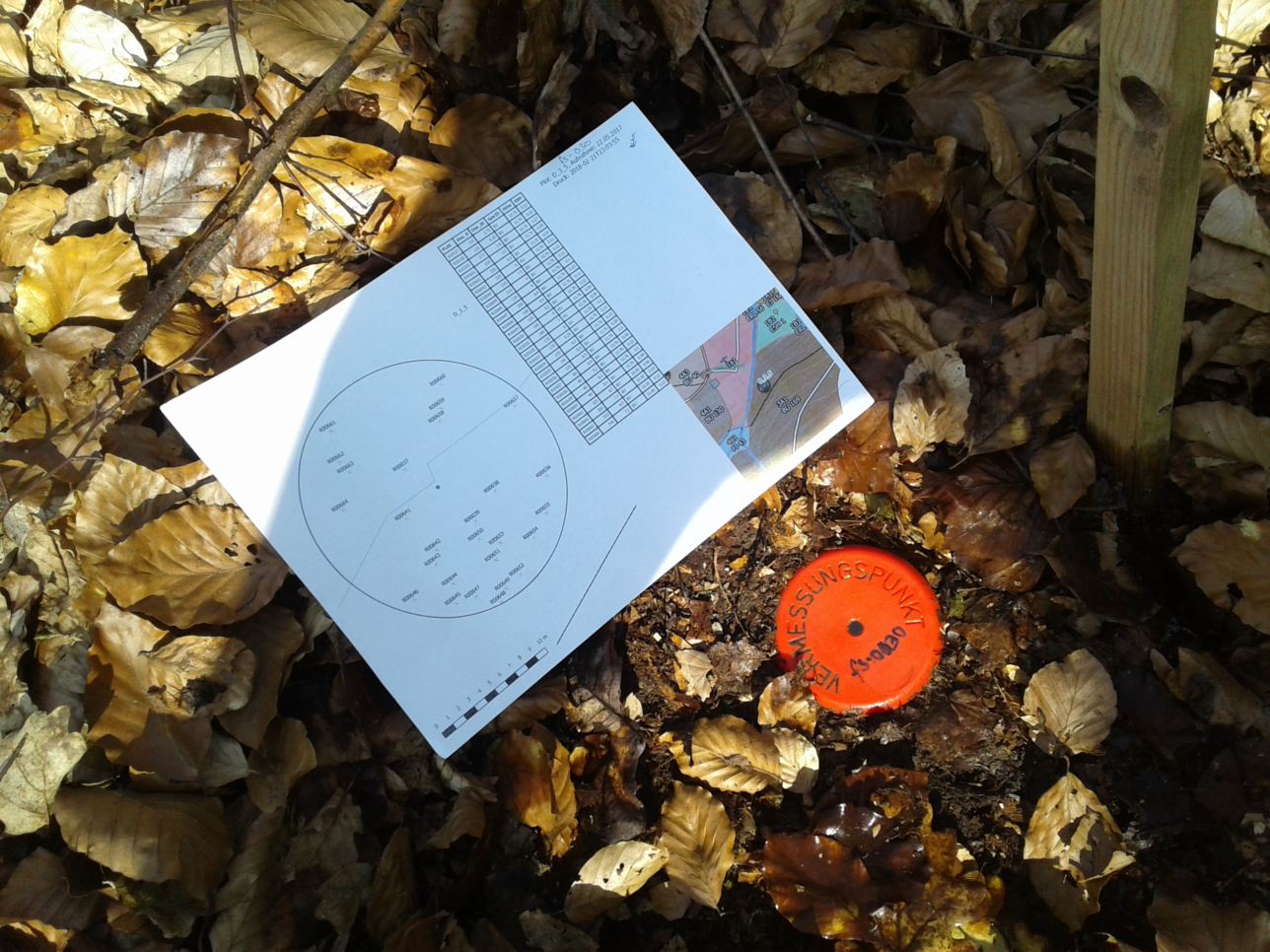
All plots are marked with a central point (stored in topopoint, see figure @ref(fig:benchmark-fig)).

On the plot following items are surveyed depending on time: * coordinates of all trees from 7 cm dbh * species * dbh * optional * height * micro habitats * vitality * social position

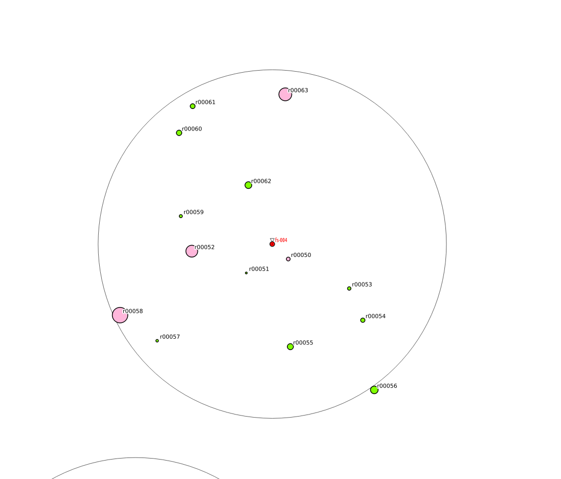
A plot from data out of MOFgeoDB is shown in figure @ref(fig:fs-plot-fig).

fs-004 as example for the visualization of the plot data in QGIS.

In real the plot looks something like this:

You can easily use R for retrievieng and visualising all plots from the github repository.

# load plots
plots <- st_read("https://github.com/MarburgOpenForest/MOFGeoDB/blob/master/MOFgeoDB.sqlite?raw=true", quiet = T, layer = "vw_plot_fs")
# alternatively from the PUM GitLab repo
#plots <- st_read("https://gitlab.uni-marburg.de/reudenba/MOFgeoDB/-/raw/master/MOFgeoDB.sqlite?raw=true", quiet = T, layer = "vw_plot_fs")

plots %>% 
  mapview(
    map.types = "OpenStreetMap", 
    color = "grey20",
    lwd = 1,
    label = plots$plot_id,
    layer.name = "fs-plots")

This will generate the below map.